Blog
How We Optimized RudderStack’s Identity Resolution Algorithm for Performance
How We Optimized RudderStack’s Identity Resolution Algorithm for Performance

Justin Driemeyer
Engineering at Rudderstack
9 min read
April 19, 2023

Identity resolution is one of the biggest barriers to generating value from customer data. The technical challenges behind unifying all user activity in one comprehensive profile are non-trivial even in basic cases. If your user journey includes multiple devices, and you want to include data from different SaaS systems in your user profiles, the task can seem insurmountable. That’s why RudderStack has always included an identity resolution feature, and it’s why we’re building our Profiles product (currently in beta). We want to make identity stitching as easy as editing a config file.
To create the identify stitching portion of the Profiles product, we started with an approach we have used before. But to make Profiles as powerful as we want it to be, we knew it needed refinement. We made some minor improvements to make it more configurable, but we needed to do more. In this post, I’ll detail how we optimized our identity stitching algorithm to meet the product requirements for Profiles while maintaining performance.
Ensuring convergence
One of the product guidelines for Profiles was that it needed to produce point-in-time correct materials. So, we needed to ensure the Identity stitcher did not allow any unconverged materials–to be point-in-time correct, the output has to be fully converged every time.
This was straightforward enough with modern SQL procedural logic: We put a loop around the stitching statement from the existing solution with a max iterations guard. After each pass through the loop, the model checks to see if any updates were made in the previous pass. If no updates were made, it knows the output is fully converged. If it detects updates, it loops again. This method reliably resulted in fully converged outputs with test datasets, but it had a critical limitation.
Unacceptably long run times
When we ran the model against real-world datasets, we discovered it was taking longer than anticipated to run. Runtime for each round was about as expected, but the loop had to run more times than anticipated to reach full convergence. The additional rounds required for full convergence with these datasets, which included hundreds of millions of unique identifiers, created a problem.
Full convergence could take multiple hours. It wasn’t out of the ordinary for a dataset to require 20 rounds of stitching to reach full convergence. At seven minutes a piece, this adds up to an unacceptably long end-to-end runtime of 140 minutes. We knew we had to make some major performance improvements, and a couple of key insights led us to a strong solution.
How we reduced runtimes by 75%
It took two steps to improve the performance of our algorithm enough to bring run times into an acceptable range. The first step was based on a more obvious insight. The second step required a keener observation and a more innovative solution.
Detect convergence and separate clusters
Our first insight was around separating converged clusters from unconverged clusters. If we could detect which edges had converged and which were still being worked on, we could move the converged clusters to a separate table at each step. By eliminating these converged clusters from the active table, the number of rows worked on would get smaller and runtime would get faster for every sequential round. Once we hit full convergence, we could simply put the tables back together. But we needed to determine how to detect which clusters had converged.
Previously we were simply checking if the table had stopped changing to detect convergence, but that wasn’t at the cluster level. The insight here was that we could first partition based on the left and right nodes of an edge to see how many distinct clusters that node was connected to. Then we could partition a second time based on cluster id. This time, we only identify that cluster as converged if all its member edges – left and right sides – were connected only to a single distinct cluster id.
Performing this second partition at the cluster level, instead of the edge level, allows us to reliably detect convergence in just two steps. As a bonus, this also simplified the test for graph convergence – if the active edges table was empty, it’s converged.
Edges don’t need to be maintained
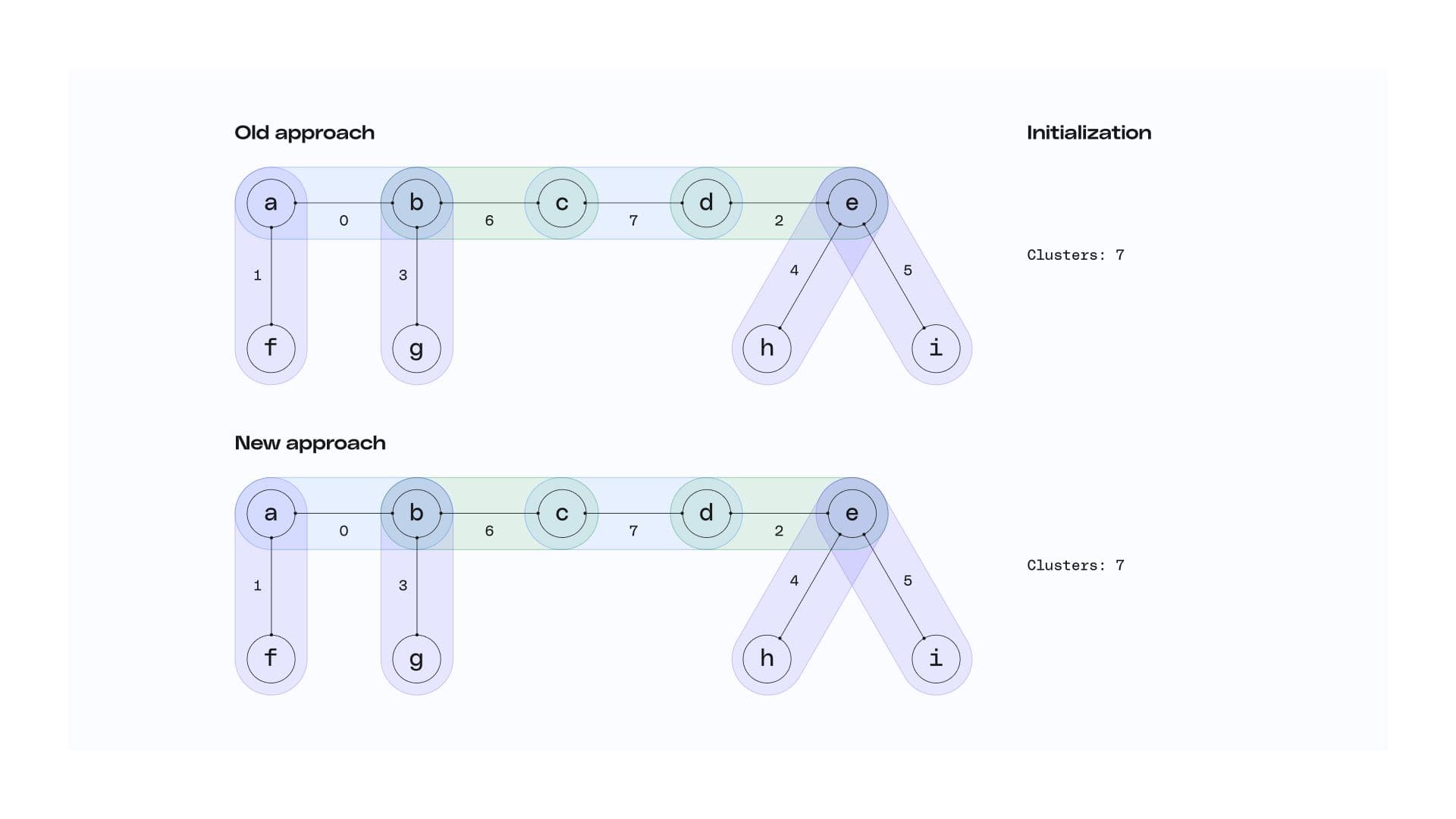
Our second insight was less obvious. A strength of our previous approach was how it avoided expensive joins through its mapping of edges to clusters. Keeping around the left and right nodes of each edge allowed us to propagate ids through the graph using two steps. First, apply a SQL window function on each side of the edge to propagate cluster ids among nodes, adding a column to each row for the left and right side of that edge with the best id for the cluster. Then, for each row, propagate across edges by just comparing those two columns.
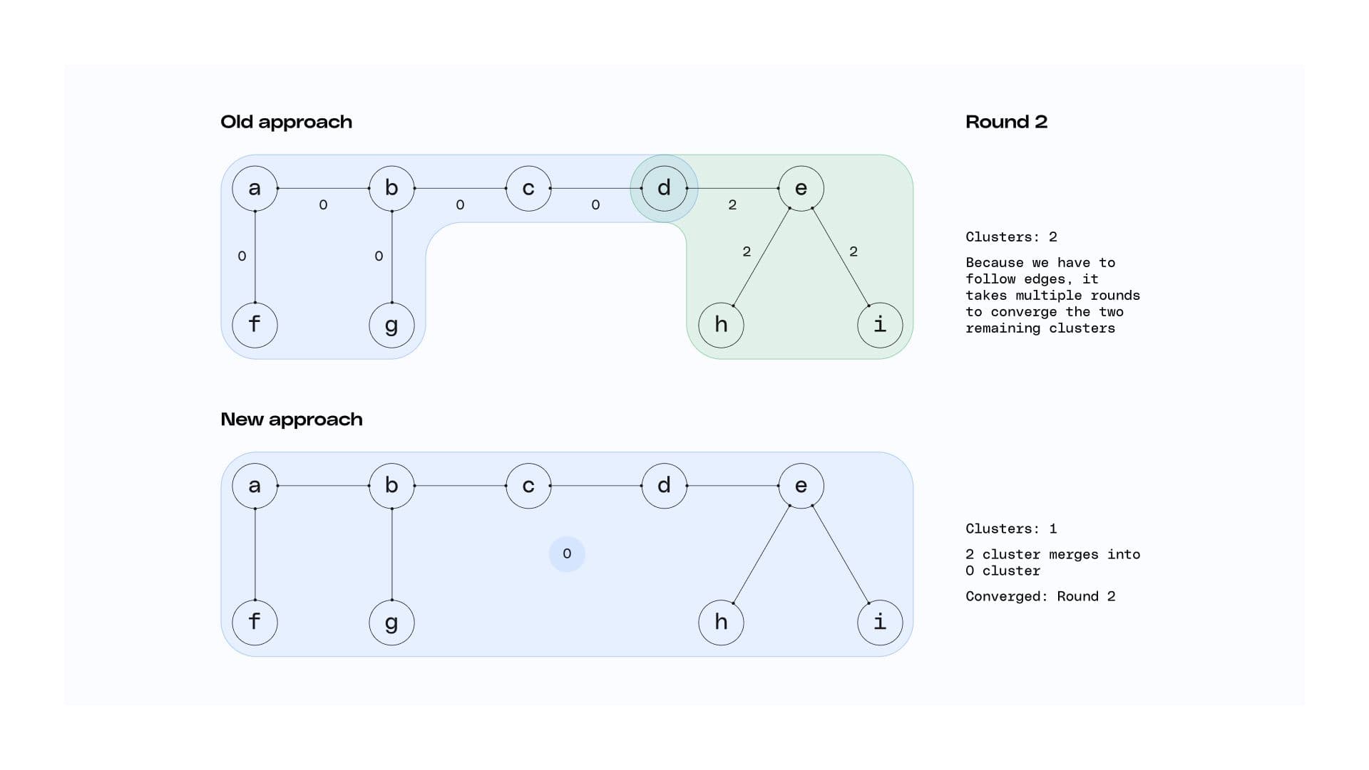
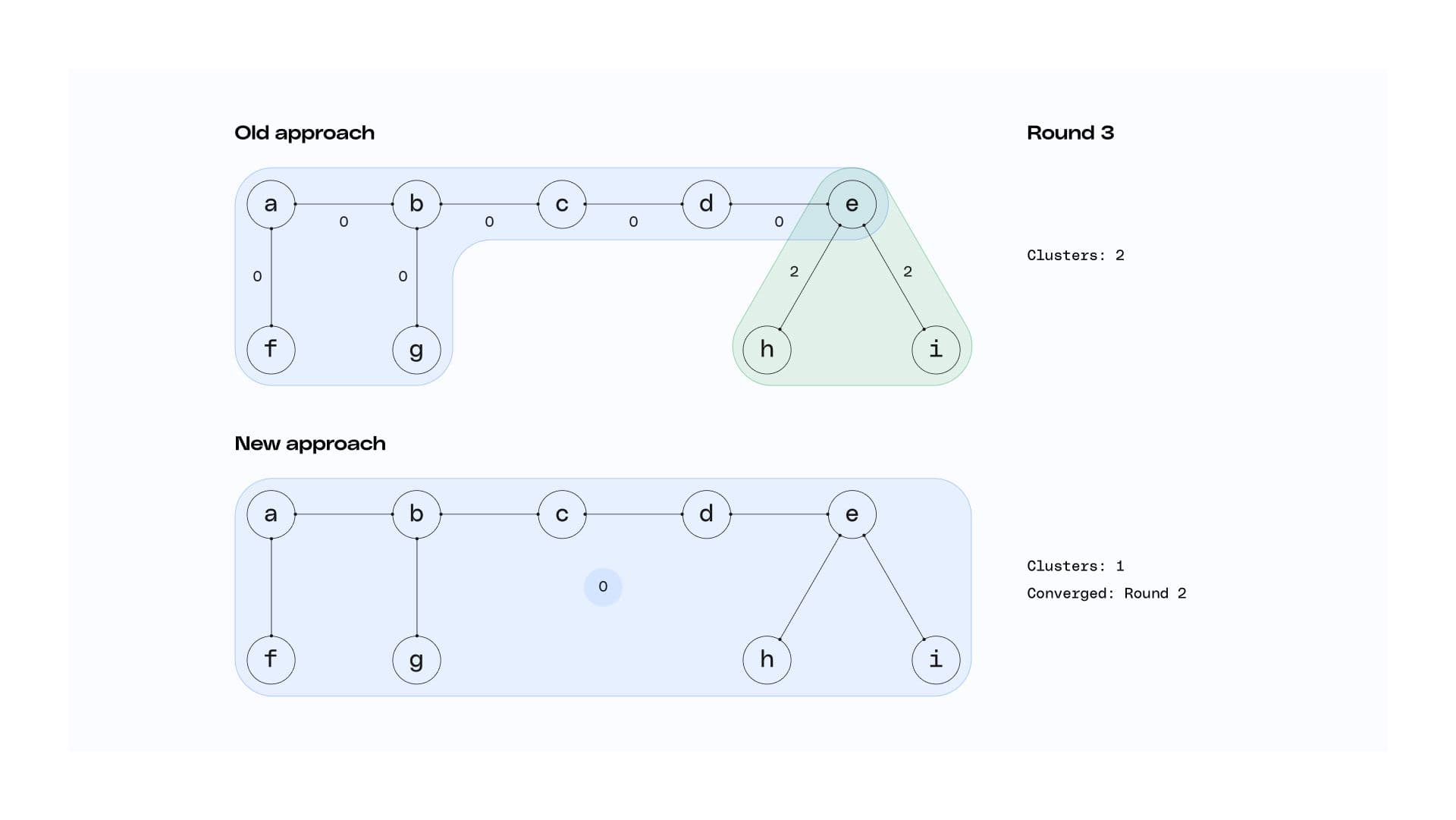
Avoiding joins this way did involve a tradeoff though. With this method, ids only propagate across edges. On an identity graph with long edges, this could take a long time and require many iterations. So, what was our second insight? Edges don’t need to be maintained.
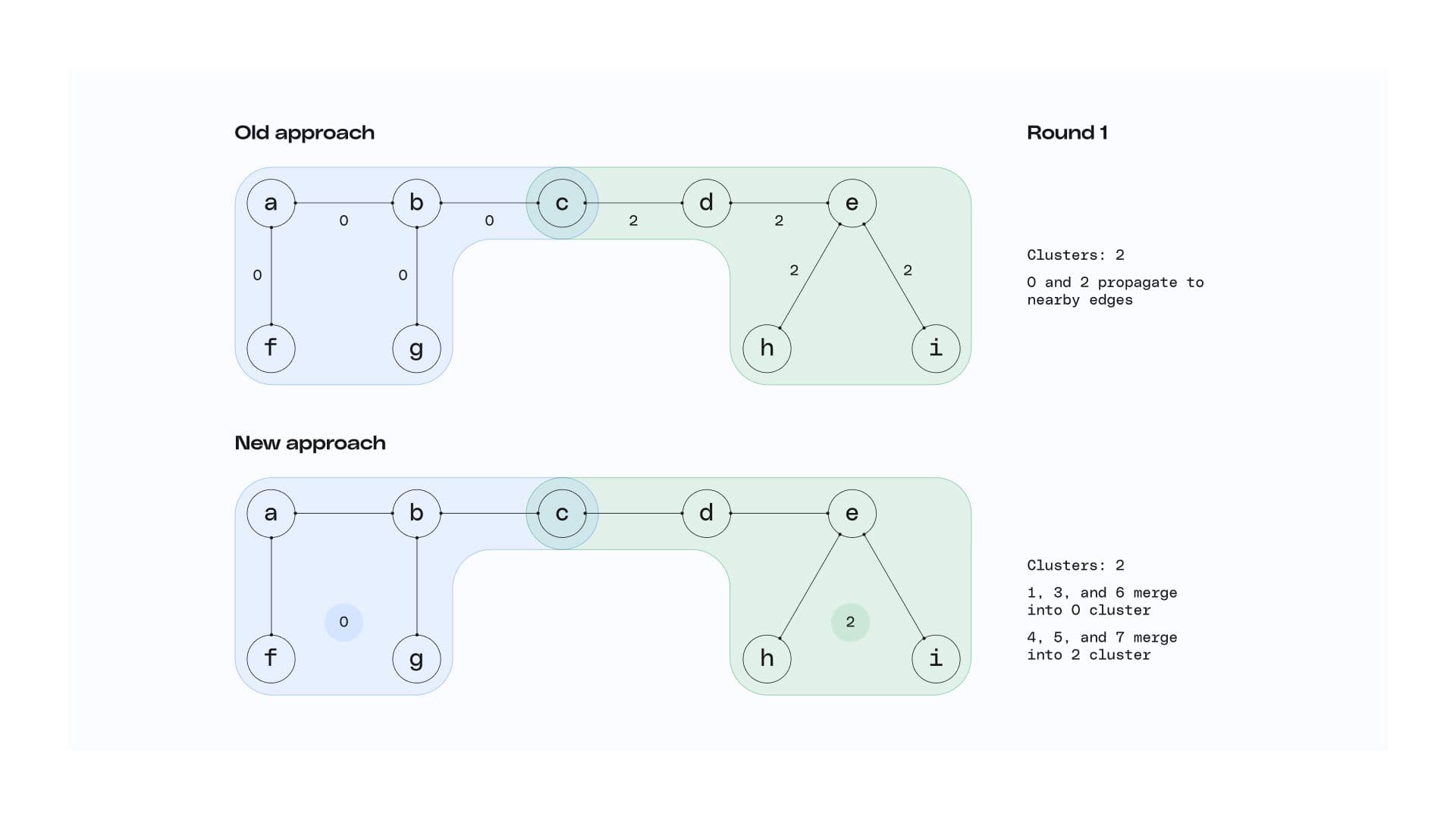
The only thing an edge tells you is that two nodes belong to the same cluster. Once that’s established, the edge is no longer strictly necessary. With this in mind, we realized we didn’t need an edge - cluster mapping table with the left and right nodes as columns. We could instead use a node - cluster mapping table and have each edge add a mini-cluster to it upon initialization. This allowed us to reframe the problem: Instead of following edges one by one, we’re progressively merging clusters. Approaching the problem this way delivers two major advantages:
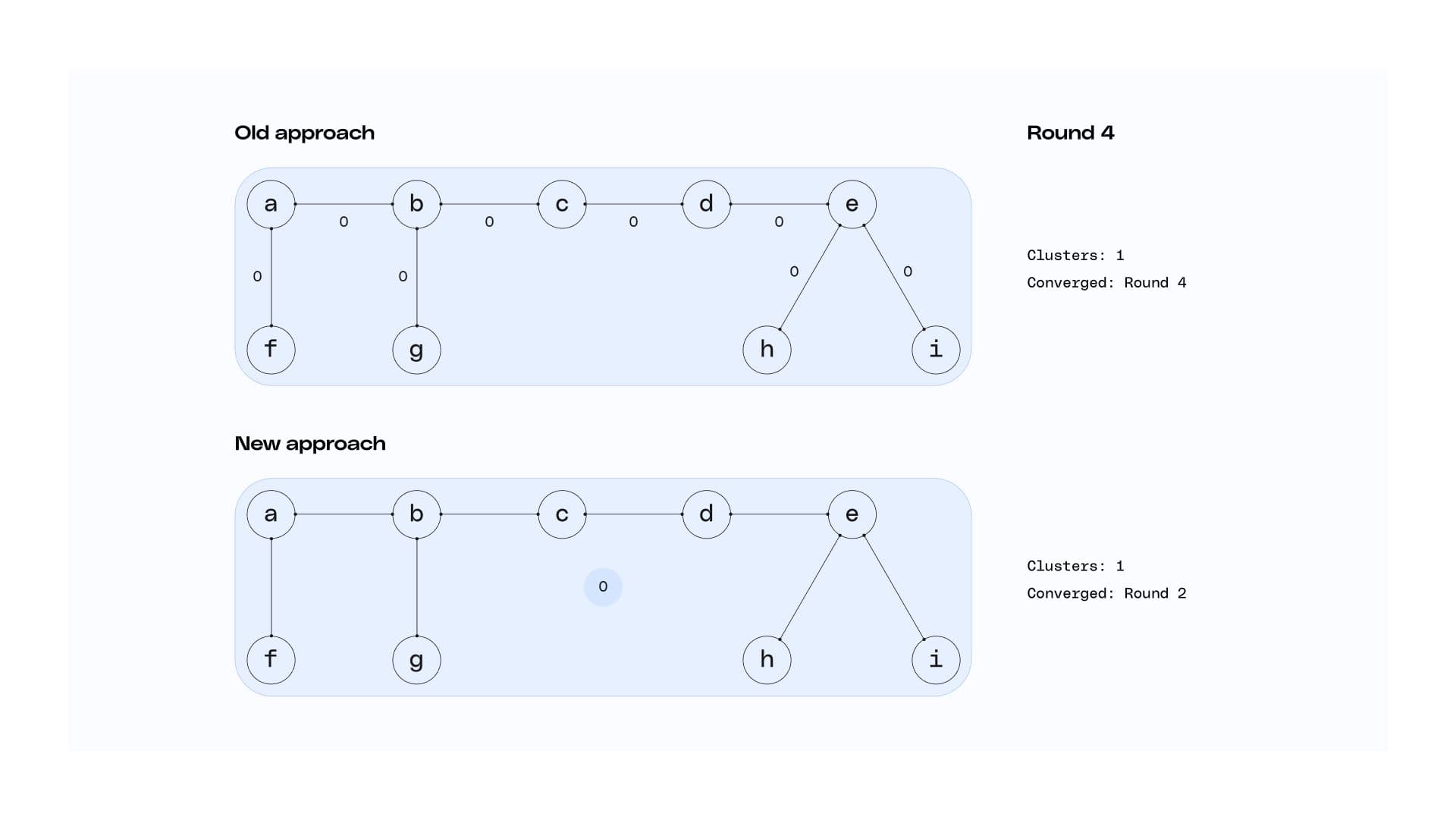
- Reduced number of steps – because every active cluster is merged into at least one other active cluster at each step, it reduces the number of steps from O(n) when following edges to O(log n) when merging clusters.
- Reduced number of active table rows each round – merging two clusters reduces the number of rows in the active mapping table. Consider two clusters in the active mapping table that are going to be merged on this iteration. There must have been at least one node that had a row for each cluster, otherwise, it would have already been converged. After merging, those rows will both have the same cluster mapping, thus the duplicate row can be removed.
So, not only are fewer steps needed, but each step is operating on a smaller table. Furthermore, the convergence check of the first insight was cluster-based, so it mapped naturally over to this approach.
Before and after
Collectively, these two optimizations delivered major performance improvements. We even built a synthetic dataset generator to prove this out. The dataset generator creates random connected component graphs with known edges, allowing us to test against random data and not bias towards any one particular real-world dataset. Our testing showed consistent, significant reductions in runtime.
Before these improvements, stitching a dataset of 100M rows with 1M unique edges, where the max cluster width was eight (so the shortest path between the two most distant connected nodes was eight) took 4 minutes and 23 seconds. After implementing these improvements, the same test took just 59 seconds, 15 of which were dedicated to parsing and compiling the queries.
There’s always more to do
This was a solid result, but there’s always opportunity to improve. One area we’ve already identified for improvement is around cold start vs. incremental mode. We already support a time-based incremental mode, and these optimizations work equally well in both the cold start and incremental cases. However, we’re currently quite conservative about building from scratch.
For instance, if a user changes a setting in their identity stitcher config, we see the change and recognize they have not run a project with these settings before. To ensure we provide accurate data, we would run that project cold start. We only use incremental mode when the identity stitcher settings haven't changed.
There’s an opportunity here for us to go further in detecting when other identity stitcher results with different settings could be used as the starting point for a future run, even when settings have changed.
Solving the technical challenges so you don’t have to
Runtime is a critical factor to the real-world usefulness of a product like Profiles. When we began building the product, we quickly realized our existing identity resolution algorithm needed some major improvements in order to meet the product requirement for point-in-time correct materials. Point-in-time correctness requires full convergence, and with our loop running upwards of twenty times to fully converge, runtimes were absolutely unacceptable.
Ultimately we were able to reduce these runtimes by 75% by making optimizations based on two significant insights that our team uncovered. Detecting convergence allowed us to separate active clusters from non-active clusters, and the realization that we did not need to maintain edges allowed us to reapproach the problem as one of merging clusters instead of following edges. With these optimizations, runs became progressively smaller at each step, and runtime dropped significantly.
Our goal in building Profiles is to solve the technical challenges of identity resolution, like the one detailed here, for you so you can focus more on making your customer profiles valuable to the business and less on the underpinning infrastructure. As we continue solving the technical challenges, we’ll continue sharing our learnings, so stay tuned for future posts. And If you’d like to join our beta, please reach out to us. We’d love your feedback.
Published:
April 19, 2023
More blog posts
Explore all blog posts
Salesforce data enrichment: Best tools for 2025
Danika Rockett
by Danika Rockett

CIAM: What is customer identity and access management?
Danika Rockett
by Danika Rockett

Deterministic vs. probabilistic models: A guide for data teams
Danika Rockett
by Danika Rockett


Start delivering business value faster
Implement RudderStack and start driving measurable business results in less than 90 days.